Just enough queueing theory to get you by

Queuing theory is a large and complex topic but it is amazing how much practical usefulness you can derive just from its basic principles. I had to learn it while undergoing my masters in computer science and it has served me well in my career when dealing with building servers and scaling them.

Understanding basic queuing theory will make it a lot easier to:

understand which bottlenecks to tackle when you are debugging a slow server;
understand the tradeoffs between optimizing code vs adding more instances;
have a solid base for sizing servers e.g adding more ram vs optimizing your garbage collector or memory layout;
read latency profile graphs and choose an SLO (service level objective) for your service.

There are a lot of concepts to understand in order to get a good grasp on queuing theory and that is why I divided this article into two parts. In part 1 (this article) will go through non-computer related examples to establish most of the concepts and in part 2 will apply them to networked servers and concepts that are more unique to them.

Credit where credit is due

I want to thank Francisco Zanfranceschi for reviewing this article and greatly helping me improve it! If you think this article is good, go thank him as well!.

Let’s go shopping!

Suppose you are the owner of a video game store here in the US. Your store has enough space to allow 30 people inside without anyone feeling uncomfortable. You measure the time a person takes inside the store to be on average 15 minutes. This includes getting in, picking what they want, getting their purchase through and then leaving the store:

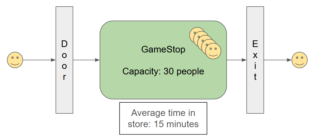
In the image above we have a diagram of the flow a customer takes:

A customer arrives at the door.
1. If the store is not full, they are allowed in.
2. If the store is full they can either wait until someone exits (they wait in a queue) or they can go away.
Once inside, they take on average 15 minutes doing whatever it is they need to do.
Once they are done, they exit the store.

Suppose, on average, that you have 1 new customer every 3 minutes (or 20 customers per hour). On average, how many people would you expect to find inside your store at any given time?

To find that number, we multiply the arrival rate (20 customers / hour) by the average service time of the customer (0.25 hours, or 15 minutes), giving you 5 customers on average. This number that we calculated, 5, is the long term average number of customers in the store L, expressed as L = λ x W, where λ (lambda) is the arrival rate and W is the service time.

Whoa, what was all that?

Amazing how in one paragraph we introduced so many concepts, right? Let’s take them one at a time:

Arrival rate (λ)

This is the number of customers arriving at the system per given unit of time. In this scenario, it’s the number of people arriving at the store door, 20 customers per hour.

Service time (W)

The amount of time a customer stays in the system. For your store, customers stay 15 minutes inside before they leave, so W is 15 minutes or 0.25 hour.

Throughput (or exit rate)

It is the number of customers that exit the system per unit of time. It is the inverse of the arrival rate, so in our scenario it’s how many people are exiting the store per unit of time.

Stable / stationary system

A system is considered stable or stationary if the arrival rate (λ) is equal to or less than the throughput (exit rate). If that holds true then, as long as the system has enough capacity, it will never have to reject a customer. For our scenario, we will assume that the throughput is equal to the arrival rate, 20 customers an hour, rendering the system stable.

L = λ x W

Conceptually simple, it is just the product (L) of the arrival rate (λ) and service time (W), resulting in the average number of customers inside a system.

This is the algebraic form of Little’s Law, which states that “the long-term average number L of customers in a stationary system is equal to the long-term average effective arrival rate λ multiplied by the average time W that a customer spends in the system”

In our scenario, L is 5 and as long as your store is stable (arrival rate <= throughput AND L <= Capacity), this value will be a measurable average number of customers inside the store.

For your store, this is the case. With 1 customer arriving every 3 minutes, once 15 minutes have passed, we have 1 client exiting for every client that enters, with 5 clients always inside the store at any given time.

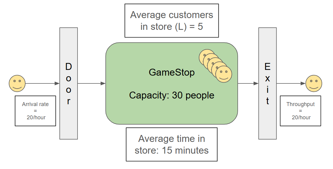
If the arrival rate was instead 3 customers per minute (180 per hour), from Little’s Law we should have L = 180 x 0.25 = 45 customers inside the store, which is much greater than its capacity of 30, making the system unstable.

In fact, at this faster arrival rate, it would take 10 minutes for the store to be full and at this point, with the current information we have available, you have 3 options: you can ask the customer to wait outside (form a queue at the door), ask new customers to come back later, or… open another store?

We must go deeper

Little’s law is remarkable, among other things, because it is composable. So, right now, we were looking at your store at a very coarse level of detail: either you are inside or not. But, you can have systems inside systems and apply the law at every level, independently of each other. So let’s do that and look at what happens inside your store.

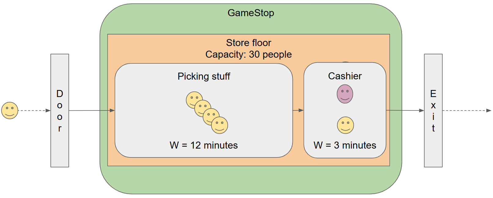
This is interesting. We now have more details about time spent in the store by customers looking around and picking their stuff (W = 12 minutes) and the time it takes for a single cashier to process the customer’s purchase (W = 3 minutes).

The original result stating the 20 customers per hour would result in a stable system still holds, since the cashier has a throughput of 20 customers per hour. But, now we know that any arrival rate higher than 20 customers per hour will result in an unstable system!

The key things in this scenario are that we have 3 different queues connected in series in this system and that each queue’s throughput (exit rate) will be the arrival rate for the next queue in the series.

Door queue

This is the entry point to the system and it’s where people arrive to enter the store. We already know the arrival rate is 20 customers per hour and as long as there is enough floor capacity available, the customer will immediately exit (pass through the door) and arrive at the next queue at 20 customers per hour rate.

Picking stuff queue

The customer is now inside the store, in the floor area and will stay inside this queue for W = 12 minutes on average, picking the stuff they want to buy. As long as there is a cashier available, the customer will, after 12 minutes, exit the picking stuff queue and go to the cashier. If there isn’t one available, the customer will wait an additional time before exiting. The exit rate (throughput) will also match the arrival rate of 20 customers per hour.

Cashier Queue

This is where the customer gets to purchase their stuff and it currently has a single cashier that takes W = 3 minutes (or 0.05 hour) to process the purchase. Because there is a single cashier, for this queue we have L = 1 customer. In order to have a stable system, the maximum arrival rate for this queue must be λ <= L(1) / W(0.05) <= 20 customers per hour, which is currently the case.

If, for example, we have 30 customers per hour (1 every 2 minutes), we could have this timeline, as shown in the image below:

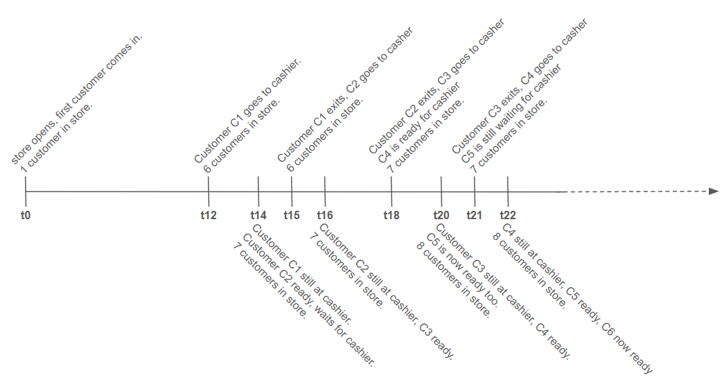
0min: Store is open, the first customer comes in.
12min: 6 customers inside the store, the first one, C1, goes to the cashier.
14min: 7 customers in the store, C2 is now ready to go to the cashier, but C1 is not done yet.
15min: 6 customers in store, C1 leaves the cashier, they can now handle C2.
16min: 7 customers in the store, C3 is ready, but has to wait for C2.
18min: 7 customers in store, C2 leaves the cashier, they can now handle C3 and C4 is ready for the cashier.
20min: 8 customers in store, C3 is not done yet, C4 is waiting and C5 is ready for the cashier.
21min: 7 customers in store, C3 leaves the cashier, they can now handle C4, C5 is still waiting.
22min: 8 customers in store, C4 still in the cashier, C5 still waiting and now C6 is ready.

As you can see, as time passes by, more and more customers become ready to be handled by the cashier, but the cashier is unable to handle them in a timely fashion. Over time, the number of customers in the store just grows until it reaches 30. At that point, the store has to ask customers to either wait at the door or go away.

Analytically, we know this because the arrival rate at the cashier (30 customers per hour) is greater than the exit rate from the cashier (20 customers per hour), making this an unstable system.

Now with more information, we can decide what can be done in order to resolve the situation.

Service time vs Throughput

Our bottleneck is the cashier. We only have 1 available and they take 3 minutes to process a purchase, a 20 customer / hour throughput. From Little’s law, we know that in order for the system to be stable, we need λ to be less than or equal to the exit rate.

We can solve this in two different ways:

Add more cashiers to the store
Have the cashier improve their purchase processing time.

Adding more cashiers (processing resources)

This is typically the easiest way to handle an unstable system. By adding a second cashier, we can double the throughput from 20 to 40 customers per hour:

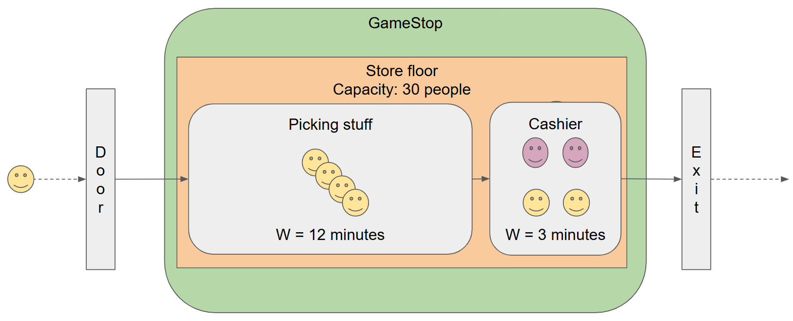
Now we can handle arrival rates of up to 1 customer every 1.5 minutes and the system will stay stable. At that rate, after 12 minutes, we would have 8 customers in the store before the first one would go to the cashier. 1.5 minutes later, a new customer comes in but an existing customer would go to the free cashier. And then every 1.5 minutes we have 1 customer exiting the store and one customer going to the cashier!

But one thing hasn’t really changed with adding a cashier. From the point of view of the customer, they are still taking 15 minutes inside the store. They still spend 12 minutes in the store on average before going to the cashier and they still spend 3 minutes with the cashier.

By adding more cashiers, you increased the throughput but the service time did not change

Improve cashier service time (optimizing resources)

With this solution, instead of adding more cashiers you give them better training, equipment and/or software such that they reduce the amount of time it takes them to process a purchase:

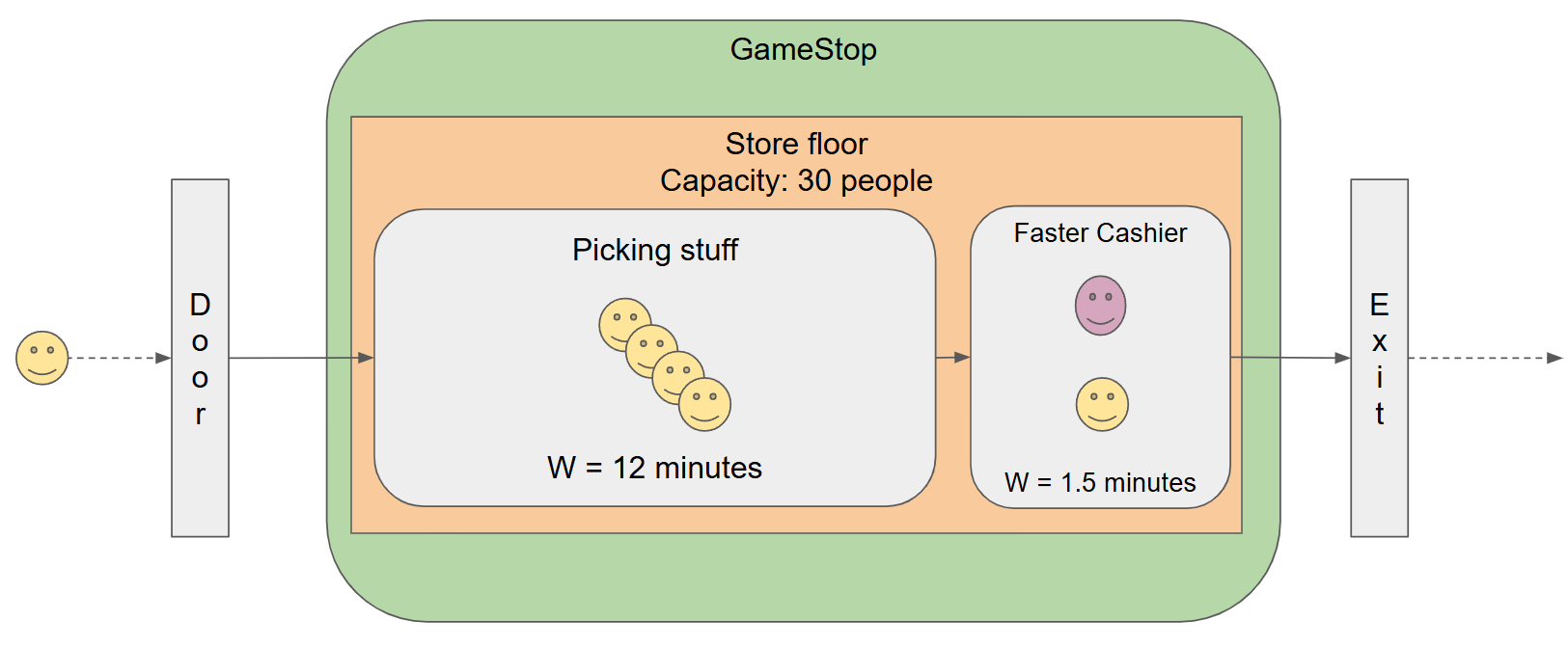
The single cashier can now process 40 customers / hour instead of 20 and thus has the same throughput as the 2 cashiers with 20 customers / hour processing. However, the total time spent in the store per customer has decreased from 15 to 13.5 minutes.

In order to achieve this throughput compared to the 2 cashier solution, more time and money had to be spent. Training takes time, better software and equipment takes time to install and iron out the problems and until the cashiers got used to the new process they might have actually increased their service time a while.

But, once done, the processing time becomes stable and now, if you add a second cashier, your processing throughput jumps from 40 to 80 customers / hour!

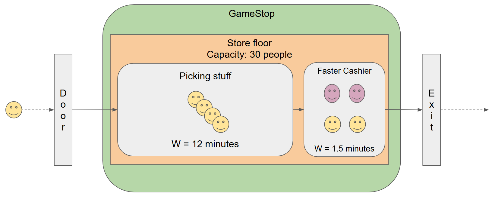
But, just like the case with the standard cashier,** adding a second faster cashier does not improve the service time for the customer**: they are still taking the same 13.5 minutes inside the store.

Store layout (space resources)

Suppose you added 6 fast cashiers, so now you can handle 240 customers per hour, or 4 customers per minute:

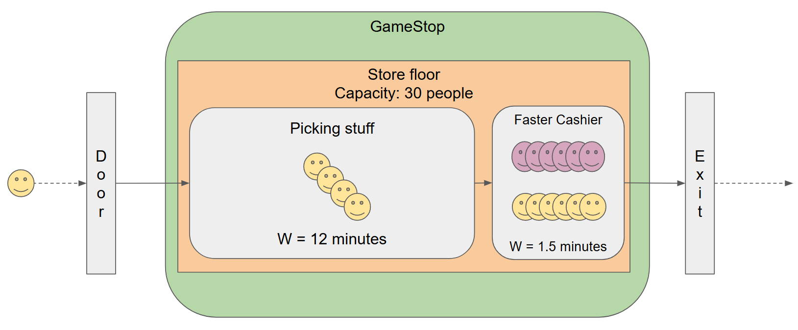
The problem now is that if we do indeed get 4 customers per minute, Little’s law tells us that the store floor customer occupation would be L = 240 x 0.2 = 48 customers, which is well above the store capacity! So, even though you have enough purchase processing capacity, you don’t have enough space for every customer that arrives and your customers will have to queue at the door or go away.

Analogous to the processing improvements, there are 2 main ways you can handle this situation:

Add more floor space
Improve floor layout.

Add more floor space (add more space resources)

If you can buy an adjacent empty store that has the same store capacity, then you can double your store floor from 30 to 60, which is 25% more than what you need to handle 240 customers / hour that need to wait 12 minutes before going to the cashier.

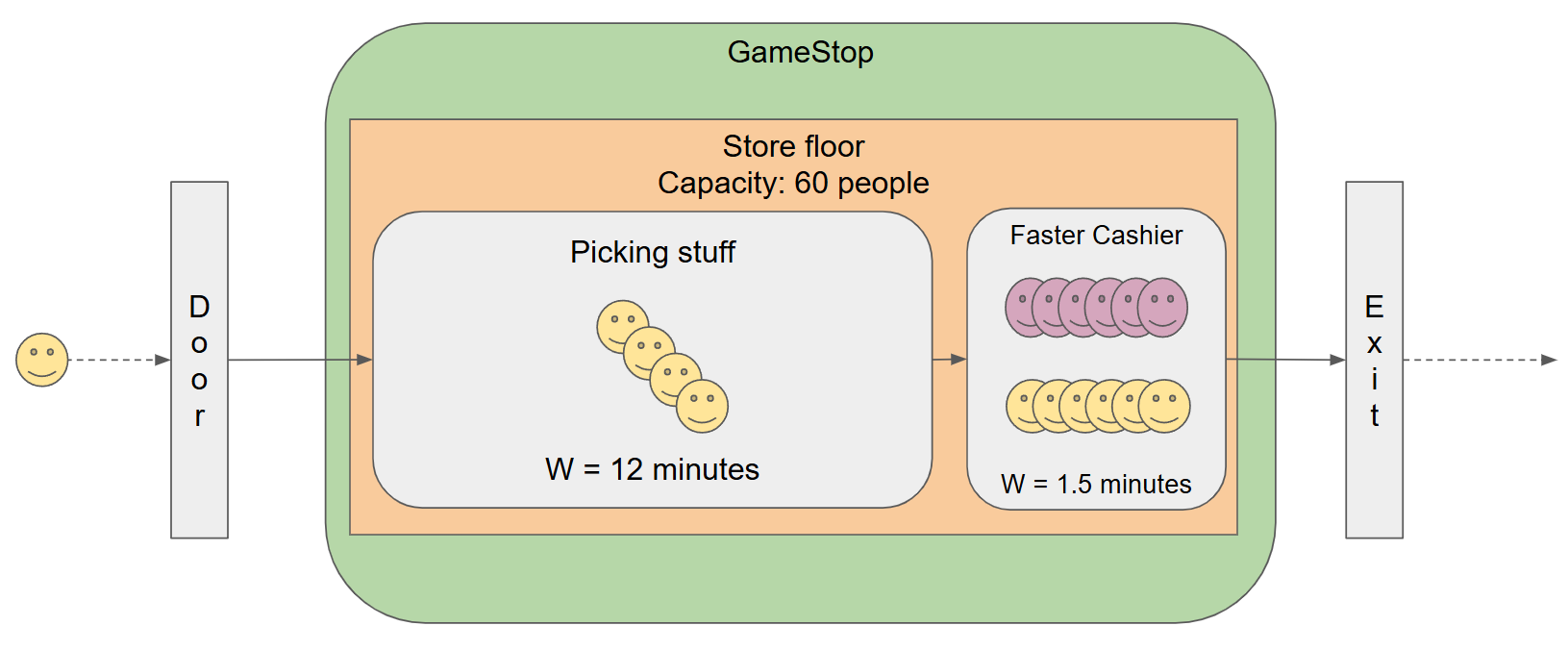
In a real world scenario, this is typically a high cost as it involves purchasing more property space. As we will see in part 2, this would be cheap for servers as it involves just adding more RAM.

Improve floor layout

By studying what your customers buy, you can

change the layout such that more common purchases are easier for them to pick out.
change the layout so they can move faster.
Group items that are typically bought together.

Once you decide and implement the changes, the average service time goes down to 6 minutes:

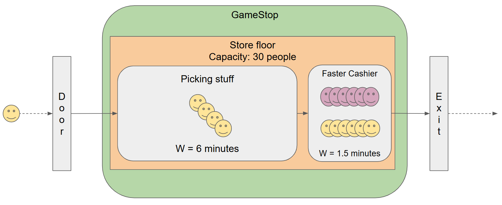
The changes meant that the service time is now also down! instead of 13.5 minutes, on average each customer is taking 7.5 minutes to get through with their purchases.

At the 4 customers / minute arrival rate, after 6 minutes there would be 24 people in the store and the first one is now ready to go to a free cashier, at the same time that a new one would come. From Little’s Law,** L = 4 x 6 = 24**, which is below your capacity of 30 customers.

For the whole system, we would have L = 4 * 7.5 = 30 and now we know the system as a whole is stable.

That was a lot, my dude!

I know, I know. Even the basics are a lot to take in at once. I hope it was easy to follow, but here is a summary of the concepts introduced here:

Arrival rate (λ) = the number of customers arriving at the system per given unit of time
Service time (W) = The amount of time a customer stays in the system.
Little’s Law (L = λ x W): the long term average number of customers inside a system, applicable only when the system is stable.
Throughput: the amount of customers that exit the system per unit of time.
Stable / stationary system: a system where the arrival rate (λ) is equal to or less than the exit rate (throughput).

In part 2, we will apply all these concepts and introduce a few more when we discuss networked services.